
2025年最佳語音轉(zhuǎn)文字API比較:一個(gè)報(bào)表31項(xiàng)指標(biāo)近200條數(shù)據(jù)
安裝依賴的命令:
pip install tensorflow matplotlib numpy pandasMNIST數(shù)據(jù)集包含60,000張訓(xùn)練圖像和10,000張測(cè)試圖像,每張為28×28像素的手寫數(shù)字灰度圖。加載數(shù)據(jù)后,建議先了解數(shù)據(jù)分布:
# 加載數(shù)據(jù)集

(train_images, train_labels), (test_images, test_labels) = mnist.load_data()


# 輸出基本信息

print(f"訓(xùn)練集維度: {train_images.shape}")  # (60000, 28, 28)

print(f"標(biāo)簽類別數(shù): {len(np.unique(train_labels))}") # 10(0-9)原始像素值范圍為0-255,直接輸入模型會(huì)導(dǎo)致數(shù)值不穩(wěn)定,歸一化(Normalization)是關(guān)鍵步驟:
# 將像素值縮放到0-1之間

train_images = train_images.astype("float32") / 255

test_images = test_images.astype("float32") / 255


# 添加通道維度(CNN要求輸入形狀為[高度, 寬度, 通道數(shù)])

train_images = np.expand_dims(train_images, -1)  # 形狀變?yōu)?60000, 28, 28, 1)

test_images = np.expand_dims(test_images, -1)


# 標(biāo)簽轉(zhuǎn)換為One-Hot編碼

num_classes = 10

train_labels = keras.utils.to_categorical(train_labels, num_classes)

test_labels = keras.utils.to_categorical(test_labels, num_classes)通過可視化樣本,檢查數(shù)據(jù)質(zhì)量并直觀理解模型的學(xué)習(xí)目標(biāo):
plt.figure(figsize=(10,5))
for i in range(15):
plt.subplot(3,5,i+1)
plt.imshow(train_images[i].squeeze(), cmap='gray') # 移除通道維度顯示圖像
plt.title(f"Label: {np.argmax(train_labels[i])}")
plt.axis('off')
plt.tight_layout()
plt.show()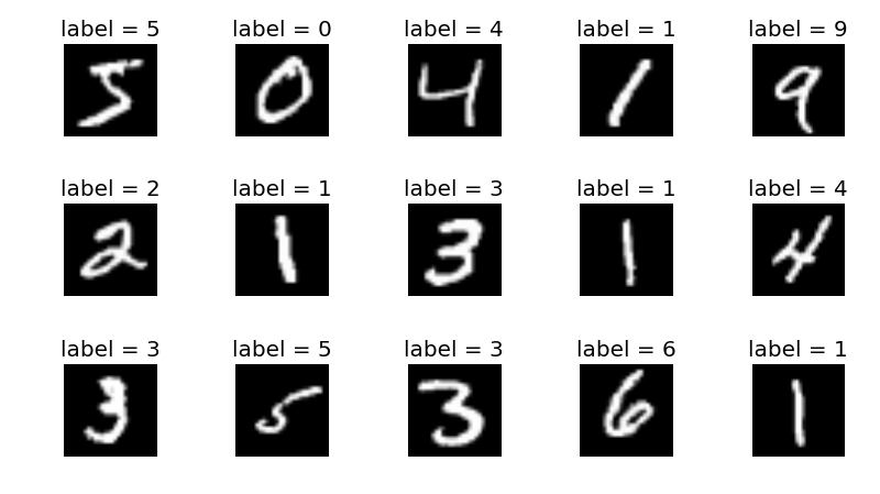 三、構(gòu)建神經(jīng)網(wǎng)絡(luò)模型
CNN通過局部感知和權(quán)值共享高效處理圖像數(shù)據(jù),核心組件包括:
model = keras.Sequential(

    [

        layers.Input(shape=(28, 28, 1)),

        # 第一卷積塊:32個(gè)3x3卷積核,ReLU激活

        layers.Conv2D(32, kernel_size=(3, 3), activation="relu"),

        layers.MaxPooling2D(pool_size=(2, 2)),  # 輸出形狀變?yōu)?13, 13, 32)

        # 第二卷積塊:64個(gè)3x3卷積核

        layers.Conv2D(64, kernel_size=(3, 3), activation="relu"),

        layers.MaxPooling2D(pool_size=(2, 2)),  # 輸出形狀(5, 5, 64)

        # 全連接層

        layers.Flatten(),  # 將3D特征展平為1D向量(5*5*64=1600)

        layers.Dropout(0.5),  # 隨機(jī)丟棄50%神經(jīng)元,防止過擬合

        layers.Dense(num_classes, activation="softmax")  # 輸出10個(gè)類別的概率

    ]

)


model.summary()  # 打印模型結(jié)構(gòu)
模型結(jié)構(gòu)輸出示例:
Total params: 34,826

Trainable params: 34,826

Non-trainable params: 0model.compile(
loss="categorical_crossentropy", # 多分類交叉熵?fù)p失函數(shù)
optimizer="adam", # 自適應(yīng)學(xué)習(xí)率優(yōu)化器
metrics=["accuracy"] # 監(jiān)控準(zhǔn)確率
)batch_size = 128 # 每次迭代使用的樣本數(shù)
epochs = 15 # 遍歷整個(gè)訓(xùn)練集的次數(shù)
history = model.fit(
train_images,
train_labels,
batch_size=batch_size,
epochs=epochs,
validation_split=0.1 # 10%訓(xùn)練數(shù)據(jù)作為驗(yàn)證集
)# 繪制訓(xùn)練曲線
plt.figure(figsize=(12, 5))
# 準(zhǔn)確率曲線
plt.subplot(1, 2, 1)
plt.plot(history.history['accuracy'], label='Training Accuracy')
plt.plot(history.history['val_accuracy'], label='Validation Accuracy')
plt.title('Accuracy Evolution')
plt.xlabel('Epoch')
plt.ylabel('Accuracy')
plt.legend()
# 損失曲線
plt.subplot(1, 2, 2)
plt.plot(history.history['loss'], label='Training Loss')
plt.plot(history.history['val_loss'], label='Validation Loss')
plt.title('Loss Evolution')
plt.xlabel('Epoch')
plt.ylabel('Loss')
plt.legend()
plt.tight_layout()
plt.show() 4.3 模型評(píng)估與過擬合判斷
score = model.evaluate(test_images, test_labels, verbose=0)

print("測(cè)試集損失:", score[0])  # 理想值應(yīng)接近驗(yàn)證損失

print("測(cè)試集準(zhǔn)確率:", score[1]) # 高于98%表明模型表現(xiàn)優(yōu)秀def predict_sample(model, image):
img = image.astype("float32") / 255
img = np.expand_dims(img, axis=0) # 添加批次維度
img = np.expand_dims(img, axis=-1) # 添加通道維度
prediction = model.predict(img)
return np.argmax(prediction)
# 隨機(jī)測(cè)試樣本預(yù)測(cè)
sample_index = np.random.randint(0, len(test_images))
plt.imshow(test_images[sample_index].squeeze(), cmap='gray')
plt.title(f"預(yù)測(cè): {predict_sample(model, test_images[sample_index])}\n真實(shí): {np.argmax(test_labels[sample_index])}")
plt.axis('off')
plt.show()# 保存完整模型(包括結(jié)構(gòu)和權(quán)重)
model.save("mnist_cnn.h5")
# 加載模型進(jìn)行推理
loaded_model = keras.models.load_model("mnist_cnn.h5")from flask import Flask, request, jsonify
import numpy as np
from PIL import Image
import io
app = Flask(__name__)
model = keras.models.load_model("mnist_cnn.h5")
@app.route('/predict', methods=['POST'])
def predict():
# 接收上傳的圖像文件
file = request.files['image']
img = Image.open(io.BytesIO(file.read())).convert('L') # 轉(zhuǎn)為灰度圖
img = img.resize((28, 28)) # 調(diào)整尺寸
# 預(yù)處理
img_array = np.array(img) / 255.0
img_array = np.expand_dims(img_array, axis=(0, -1)) # 添加批次和通道維度
# 預(yù)測(cè)并返回結(jié)果
prediction = model.predict(img_array)
return jsonify({'prediction': int(np.argmax(prediction))})
if __name__ == '__main__':
app.run(host='0.0.0.0', port=5000)測(cè)試API:
curl -X POST -F "image=@test_image.png" http://localhost:5000/predict

# 預(yù)期返回:{"prediction": 7}from keras.preprocessing.image import ImageDataGenerator
datagen = ImageDataGenerator(rotation_range=10, zoom_range=0.1)
model.fit(datagen.flow(train_images, train_labels, batch_size=32))learning_rate。通過本教程,你已掌握了使用Python和Keras開發(fā)AI模型的完整流程。從數(shù)據(jù)預(yù)處理到模型部署,每個(gè)環(huán)節(jié)都至關(guān)重要。建議在實(shí)際項(xiàng)目中嘗試調(diào)整模型結(jié)構(gòu)(如增加LSTM處理時(shí)序數(shù)據(jù)),或探索更復(fù)雜的應(yīng)用場(chǎng)景(如目標(biāo)檢測(cè))。記住,持續(xù)實(shí)踐和參與開源社區(qū)是提升技能的最佳途徑。
2025年最佳語音轉(zhuǎn)文字API比較:一個(gè)報(bào)表31項(xiàng)指標(biāo)近200條數(shù)據(jù)
微信截圖_17436524948840.png)
每個(gè) API 團(tuán)隊(duì)都應(yīng)該知道的十大 API 安全威脅
微信截圖_17435904448874.png)
跟大牛學(xué)LLM訓(xùn)練和使用技巧
鍵.png)
如何使用 Natural Language API 進(jìn)行實(shí)體和情感分析

GLM-4 智能對(duì)話機(jī)器人本地部署指南

Krea AI核心功能揭秘:從圖像生成到模型訓(xùn)練

如何使用Requests-OAuthlib實(shí)現(xiàn)OAuth認(rèn)證
2025年最新LangChain Agent教程:從入門到精通
Python實(shí)現(xiàn)五子棋AI對(duì)戰(zhàn)的詳細(xì)教程
對(duì)比大模型API的內(nèi)容創(chuàng)意新穎性、情感共鳴力、商業(yè)轉(zhuǎn)化潛力
一鍵對(duì)比試用API 限時(shí)免費(fèi)