如何快速實現(xiàn)REST API集成以優(yōu)化業(yè)務(wù)流程
device = (

    "mps"

    if torch.backends.mps.is_available()

    else "cuda"

    if torch.cuda.is_available()

    else "cpu"

)
# 載入一個預(yù)訓(xùn)練過的管線
pipeline_name = "johnowhitaker/sd-class-wikiart-from-bedrooms"
image_pipe = DDPMPipeline.from_pretrained(pipeline_name).to(device)
# 使用DDIM調(diào)度器,僅用40步生成一些圖片
scheduler = DDIMScheduler.from_pretrained(pipeline_name)
scheduler.set_timesteps(num_inference_steps=40)
# 將隨機(jī)噪聲作為出發(fā)點(diǎn)
x = torch.randn(8, 3, 256, 256).to(device)
# 使用一個最簡單的采樣循環(huán)
for i, t in tqdm(enumerate(scheduler.timesteps)):
model_input = scheduler.scale_model_input(x, t)
with torch.no_grad():
noise_pred = image_pipe.unet(model_input, t)["sample"]
x = scheduler.step(noise_pred, t, x).prev_sample
# 查看生成結(jié)果,如圖5-10所示
grid = torchvision.utils.make_grid(x, nrow=4)
plt.imshow(grid.permute(1, 2, 0).cpu().clip(-1, 1) * 0.5 + 0.5)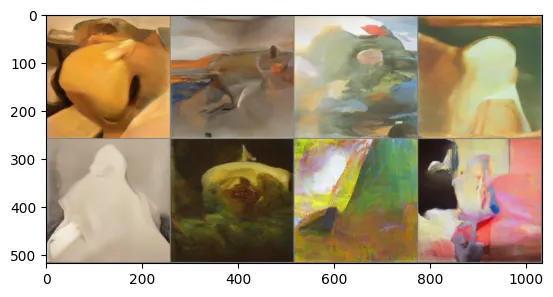
? ?正如上圖所示,模型可以生成一些圖片,那么如何進(jìn)行控制輸出呢?下面我們以控制圖片生成綠色風(fēng)格為例介紹AIGC模型控制:
? ? ? ?思路是:定義一個均方誤差損失函數(shù),讓生成的圖片像素值盡量接近目標(biāo)顏色;
def color_loss(images, target_color=(0.1, 0.9, 0.5)):

    """給定一個RGB值,返回一個損失值,用于衡量圖片的像素值與目標(biāo)顏色相差多少;

 這里的目標(biāo)顏色是一種淺藍(lán)綠色,對應(yīng)的RGB值為(0.1, 0.9, 0.5)"""

    target = (

        torch.tensor(target_color).to(images.device) * 2 - 1

    )  # 首先對target_color進(jìn)行歸一化,使它的取值區(qū)間為(-1, 1)

    target = target[

        None, :, None, None

    ]  # 將所生成目標(biāo)張量的形狀改為(b, c, h, w),以適配輸入圖像images的

 # 張量形狀

    error = torch.abs(

        images - target

    ).mean()  # 計算圖片的像素值以及目標(biāo)顏色的均方誤差

    return error
接下來,需要修改采樣循環(huán)操作,具體操作步驟如下:
方法一:從UNet中獲取噪聲預(yù)測,并將輸入圖像X的requires_grad屬性設(shè)置為True,這樣可以充分利用內(nèi)存(因為不需要通過擴(kuò)散模型追蹤梯度),但是這會導(dǎo)致梯度的精度降低;
方法二:先將輸入圖像X的requires_grad屬性設(shè)置為True,然后傳遞給UNet并計算“去噪”后的圖像X0;
下面分別看一下這兩種方法的效果:
# 第一種方法


# guidance_loss_scale用于決定引導(dǎo)的強(qiáng)度有多大

guidance_loss_scale = 40  # 可設(shè)定為5~100的任意數(shù)字


x = torch.randn(8, 3, 256, 256).to(device)


for i, t in tqdm(enumerate(scheduler.timesteps)):


    # 準(zhǔn)備模型輸入

    model_input = scheduler.scale_model_input(x, t)


    # 預(yù)測噪聲

    with torch.no_grad():

        noise_pred = image_pipe.unet(model_input, t)["sample"]


    # 設(shè)置x.requires_grad為True

    x = x.detach().requires_grad_()


    # 得到“去噪”后的圖像

    x0 = scheduler.step(noise_pred, t, x).pred_original_sample


    # 計算損失值

    loss = color_loss(x0) * guidance_loss_scale

    if i % 10 == 0:

        print(i, "loss:", loss.item())


    # 獲取梯度

    cond_grad = -torch.autograd.grad(loss, x)[0]


    # 使用梯度更新x

    x = x.detach() + cond_grad


    # 使用調(diào)度器更新x

    x = scheduler.step(noise_pred, t, x).prev_sample

# 查看結(jié)果

grid = torchvision.utils.make_grid(x, nrow=4)

im = grid.permute(1, 2, 0).cpu().clip(-1, 1) * 0.5 + 0.5

Image.fromarray(np.array(im * 255).astype(np.uint8))
# 輸出
0 loss: 29.37018394470215
10 loss: 12.116650581359863
20 loss: 11.641704559326172
30 loss: 11.78276252746582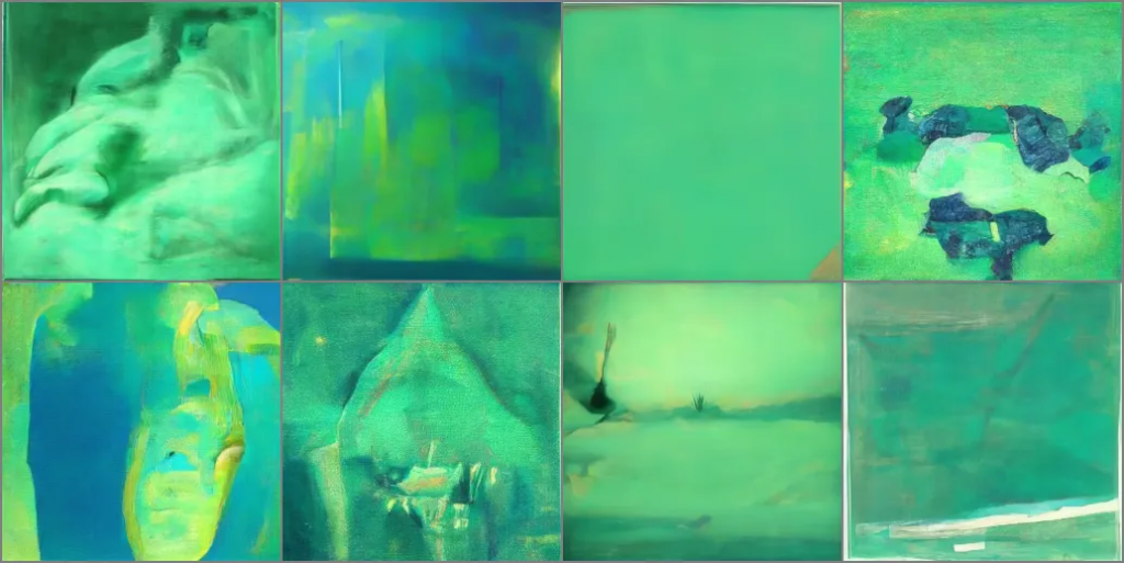
# 第二種方法:在模型預(yù)測前設(shè)置好x.requires_grad

guidance_loss_scale = 40

x = torch.randn(4, 3, 256, 256).to(device)


for i, t in tqdm(enumerate(scheduler.timesteps)):


    # 首先設(shè)置好requires_grad

    x = x.detach().requires_grad_()

    model_input = scheduler.scale_model_input(x, t)


    # 預(yù)測

    noise_pred = image_pipe.unet(model_input, t)["sample"]


    # 得到“去噪”后的圖像

    x0 = scheduler.step(noise_pred, t, x).pred_original_sample


    # 計算損失值

    loss = color_loss(x0) * guidance_loss_scale

    if i % 10 == 0:

        print(i, "loss:", loss.item())


    # 獲取梯度

    cond_grad = -torch.autograd.grad(loss, x)[0]


    # 根據(jù)梯度修改x

    x = x.detach() + cond_grad


    # 使用調(diào)度器更新x

    x = scheduler.step(noise_pred, t, x).prev_sample


grid = torchvision.utils.make_grid(x, nrow=4)

im = grid.permute(1, 2, 0).cpu().clip(-1, 1) * 0.5 + 0.5

Image.fromarray(np.array(im * 255).astype(np.uint8))
# 輸出
0 loss: 27.62268829345703
10 loss: 16.842506408691406
20 loss: 15.54642105102539
30 loss: 15.545379638671875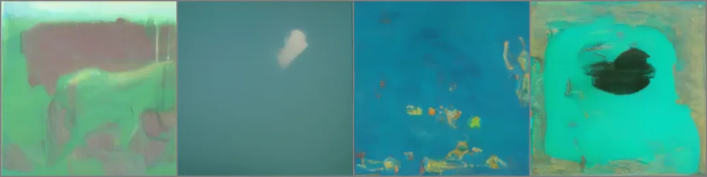
從上圖看出,第二種方法效果略差,但是第二種方法的輸出更接近訓(xùn)練模型所使用的數(shù)據(jù),也可以通過修改guidance_loss_scale參數(shù)來增強(qiáng)顏色的遷移效果。
? ? ? ?雖然上述方式可以引導(dǎo)和控制圖像生成某種顏色,但現(xiàn)在LLM更主流的方式是通過Prompt(僅僅打幾行字描述需求)來得到自己想要的圖像,那么CLIP是一個不錯的選擇。CLIP是有OpenAI開發(fā)的圖文匹配大模型,由于這個過程是可微分的,所以可以將其作為損失函數(shù)來引導(dǎo)擴(kuò)散模型。
import open_clip


clip_model, _, preprocess = open_clip.create_model_and_transforms(

    "ViT-B-32", pretrained="openai"

)

clip_model.to(device)


# 圖像變換:用于修改圖像尺寸和增廣數(shù)據(jù),同時歸一化數(shù)據(jù),以使數(shù)據(jù)能夠適配CLIP模型

tfms = torchvision.transforms.Compose(

    [

        torchvision.transforms.RandomResizedCrop(224),# 隨機(jī)裁剪

        torchvision.transforms.RandomAffine(5),       # 隨機(jī)扭曲圖片

        torchvision.transforms.RandomHorizontalFlip(),# 隨機(jī)左右鏡像,

 # 你也可以使用其他增廣方法

        torchvision.transforms.Normalize(

            mean=(0.48145466, 0.4578275, 0.40821073),

            std=(0.26862954, 0.26130258, 0.27577711),

        ),

    ]

)


# 定義一個損失函數(shù),用于獲取圖片的特征,然后與提示文字的特征進(jìn)行對比

def clip_loss(image, text_features):

    image_features = clip_model.encode_image(

        tfms(image)

    )  # 注意施加上面定義好的變換

    input_normed = torch.nn.functional.normalize(image_features.

       unsqueeze(1), dim=2)

    embed_normed = torch.nn.functional.normalize(text_features.

       unsqueeze(0), dim=2)

    dists = (

        input_normed.sub(embed_normed).norm(dim=2).div(2).

           arcsin().pow(2).mul(2)

    )  # 使用Squared Great Circle Distance計算距離

return dists.mean()?下面是引導(dǎo)模型生成圖像的過程,步驟與上述類似,只需要把color_loss()替換成CLIP的損失函數(shù)
prompt = "Red Rose (still life), red flower painting"


# 讀者可以探索一下這些超參數(shù)的影響

guidance_scale = 8

n_cuts = 4


# 這里使用稍微多一些的步數(shù)

scheduler.set_timesteps(50)


# 使用CLIP從提示文字中提取特征

text = open_clip.tokenize([prompt]).to(device)

with torch.no_grad(), torch.cuda.amp.autocast():

    text_features = clip_model.encode_text(text)


x = torch.randn(4, 3, 256, 256).to(

    device

)


for i, t in tqdm(enumerate(scheduler.timesteps)):


    model_input = scheduler.scale_model_input(x, t)


    # 預(yù)測噪聲

    with torch.no_grad():

        noise_pred = image_pipe.unet(model_input, t)["sample"]


    cond_grad = 0


    for cut in range(n_cuts):


        # 設(shè)置輸入圖像的requires_grad屬性為True

        x = x.detach().requires_grad_()


        # 獲得“去噪”后的圖像

        x0 = scheduler.step(noise_pred, t, x).pred_original_sample


        # 計算損失值

        loss = clip_loss(x0, text_features) * guidance_scale


        # 獲取梯度并使用n_cuts進(jìn)行平均

        cond_grad -= torch.autograd.grad(loss, x)[0] / n_cuts


    if i % 25 == 0:

        print("Step:", i, ", Guidance loss:", loss.item())


    # 根據(jù)這個梯度更新x

    alpha_bar = scheduler.alphas_cumprod[i]

    x = (

        x.detach() + cond_grad * alpha_bar.sqrt()

    )  # 注意這里的縮放因子


    # 使用調(diào)度器更新x

    x = scheduler.step(noise_pred, t, x).prev_sample


grid = torchvision.utils.make_grid(x.detach(), nrow=4)

im = grid.permute(1, 2, 0).cpu().clip(-1, 1) * 0.5 + 0.5

Image.fromarray(np.array(im * 255).astype(np.uint8))
# 輸出
Step: 0 , Guidance loss: 7.418107986450195
Step: 25 , Guidance loss: 7.085518836975098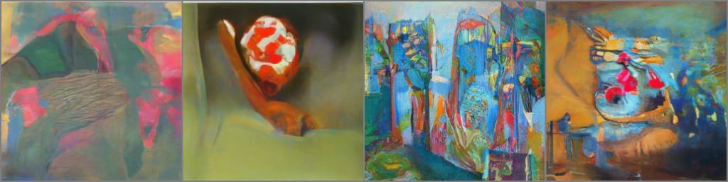
?? ?上述生成的圖像雖然不夠完美,但可以調(diào)整一些超參數(shù),比如梯度縮放因子alpha_bar.sqrt(),雖然理論上存在所謂的正確的縮放這些梯度方法,但在實踐中仍需要實驗來檢驗,下面介紹一些常用的方案:
plt.plot([1 for a in scheduler.alphas_cumprod], label="no scaling")

plt.plot([a for a in scheduler.alphas_cumprod], label="alpha_bar")

plt.plot([a.sqrt() for a in scheduler.alphas_cumprod],

    label="alpha_bar.sqrt()")

plt.plot(

    [(1 - a).sqrt() for a in scheduler.alphas_cumprod], label="(1-

     alpha_bar).sqrt()"

)

plt.legend()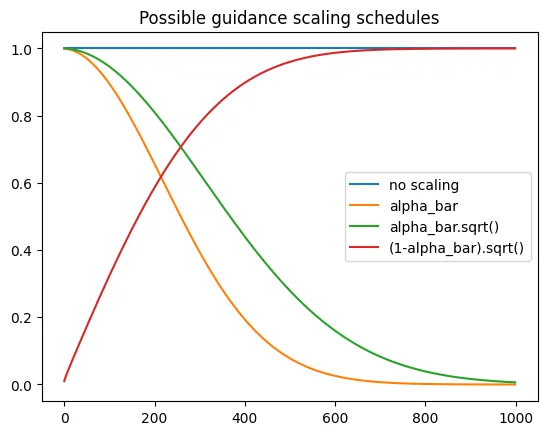
文章轉(zhuǎn)自微信公眾號@ArronAI


鍵.png)